Tutorial 4: Analyzing Topographic Models
In this tutorial we explore the results of a trained MuTopia topographic model. We will:
Load a trained model and annotate a G-Tensor with component weights and SHAP values
Visualize mutational signatures (SBS spectra) for each component
Summarize feature importance with SHAP plots
Build genome-browser track views comparing predicted and observed mutation rates
Inspect component interactions with the feature interaction matrix
Prerequisites: Tutorial 3 (Training Models). You should have:
tutorial_data/trained_model.pkl— a trained topographic modeltutorial_data/Liver.nc— the annotated G-Tensor dataset
[1]:
import mutopia.analysis as mu
import mutopia.plot.track_plot as tr
import matplotlib.pyplot as plt

model = mu.load_model('tutorial_data/pretrained_model.pkl')
print(model)
/Users/allen/miniconda3/envs/mutopia-model/lib/python3.12/site-packages/tqdm/auto.py:21: TqdmWarning: IProgress not found. Please update jupyter and ipywidgets. See https://ipywidgets.readthedocs.io/en/stable/user_install.html
  from .autonotebook import tqdm as notebook_tqdm
INFO     Mutopia JIT-compiling model operations ...
SBSModel(convolution_width=1, eval_every=5, l2_regularization=0.0,
         locus_subsample=0.125, max_features=0.5, seed=110, threads=5)
1. Annotate the G-Tensor
annot_data runs all annotation steps in one call: component contributions, local variable predictions, marginal mutation rate predictions, and SHAP feature attributions. Set calc_shap=True to also compute SHAP values (takes a few minutes; increase threads to speed it up).
[2]:
data = mu.gt.load_dataset('tutorial_data/Liver.nc', with_samples=False)
data = model.annot_data(data, threads=4, calc_shap=True)
print(data)
INFO     Mutopia Setting up dataset state ...
INFO     Mutopia Done ...
INFO     Mutopia Setting model to prediction mode.
Estimating contributions: 100%|██████████████████████████████████| 185/185 [00:01<00:00, 157.51it/s]
INFO     Mutopia Added key to dataset: "contributions"
INFO     Mutopia Added keys to dataset: Spectra/spectra, Spectra/interactions, Spectra/shared_effects
INFO     Mutopia Calculating SHAP values for M0 ...
INFO     Mutopia Calculating SHAP values for M1 ...
INFO     Mutopia Calculating SHAP values for M2 ...
INFO     Mutopia Calculating SHAP values for M3 ...
 20%|====                | 396/2000 [00:22<01:29]       IOStream.flush timed out

 50%|==========          | 1005/2000 [02:00<01:58]       INFO     Mutopia Calculating SHAP values for M4 ...
 51%|==========          | 1025/2000 [02:16<02:09]       IOStream.flush timed out
 89%|==================  | 1774/2000 [02:39<00:20]       IOStream.flush timed out
 54%|===========         | 1074/2000 [02:27<02:06]       INFO     Mutopia Calculating SHAP values for M5 ...
 67%|=============       | 1339/2000 [02:11<01:04]       INFO     Mutopia Calculating SHAP values for M6 ...
 71%|==============      | 1421/2000 [02:26<00:59]       IOStream.flush timed outIOStream.flush timed out

 81%|================    | 1613/2000 [02:55<00:41]       INFO     Mutopia Calculating SHAP values for M7 ...
 81%|================    | 1617/2000 [03:10<00:45]       IOStream.flush timed out
IOStream.flush timed out
 34%|=======             | 670/2000 [00:52<01:43]       INFO     Mutopia Calculating SHAP values for M8 ...
 42%|========            | 839/2000 [01:39<02:16]       INFO     Mutopia Calculating SHAP values for M9 ...
 45%|=========           | 893/2000 [01:52<02:18]       IOStream.flush timed outIOStream.flush timed out

 12%|==                  | 234/2000 [00:12<01:30]       IOStream.flush timed out
 35%|=======             | 708/2000 [01:20<02:25]       IOStream.flush timed out
 12%|==                  | 235/2000 [00:23<02:52]
 69%|==============      | 1380/2000 [03:06<01:23]       INFO     Mutopia Calculating SHAP values for M10 ...
 18%|====                | 354/2000 [00:11<00:51]       IOStream.flush timed out
 82%|================    | 1646/2000 [04:19<00:55]       IOStream.flush timed out
 96%|=================== | 1925/2000 [03:10<00:07]       IOStream.flush timed out
 76%|===============     | 1520/2000 [03:44<01:10]       INFO     Mutopia Calculating SHAP values for M11 ...
 20%|====                | 395/2000 [00:11<00:44]       IOStream.flush timed out
IOStream.flush timed out
IOStream.flush timed out
 78%|================    | 1551/2000 [04:09<01:12]       INFO     Mutopia Calculating SHAP values for M12 ...
 26%|=====               | 522/2000 [00:26<01:13]       IOStream.flush timed out
 64%|=============       | 1276/2000 [01:48<01:01]       INFO     Mutopia Calculating SHAP values for M13 ...
 50%|==========          | 1008/2000 [01:28<01:26]       IOStream.flush timed out
 56%|===========         | 1127/2000 [02:42<02:05]       IOStream.flush timed outIOStream.flush timed out

 37%|=======             | 735/2000 [01:15<02:09]       INFO     Mutopia Calculating SHAP values for M14 ...
 75%|===============     | 1500/2000 [02:57<00:59]       IOStream.flush timed out

 99%|===================| 1979/2000 [03:25<00:02]        INFO     Mutopia Added key: "SHAP_values"
INFO     Mutopia Added key: "component_distributions"
INFO     Mutopia Added key: "component_distributions_locus"
INFO     Mutopia Added key: "predicted_marginal"
INFO     Mutopia Added key: "predicted_marginal_locus"
Reducing samples: 100%|██████████| 184/184 [00:27<00:00,  6.77it/s]
INFO     Mutopia Added key: "empirical_marginal"
INFO     Mutopia Added key: "empirical_marginal_locus"
<mutopia.gtensor.interfaces.CorpusInterface object at 0x32d573b50>
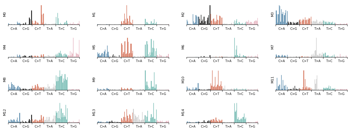
2. Visualize Mutational Signatures
Each component learns a mutational signature — the probability distribution over SBS trinucleotide contexts. plot_signature_panel shows all components side by side.
[3]:
mu.pl.plot_signature_panel(data)
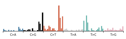
[4]:
components = mu.gt.list_components(data)
print('Discovered components:', components)

# Zoom into a single component
mu.pl.plot_component(data, components[0])
Discovered components: [np.str_('M0'), np.str_('M1'), np.str_('M2'), np.str_('M3'), np.str_('M4'), np.str_('M5'), np.str_('M6'), np.str_('M7'), np.str_('M8'), np.str_('M9'), np.str_('M10'), np.str_('M11'), np.str_('M12'), np.str_('M13'), np.str_('M14')]
[4]:
<Axes: >
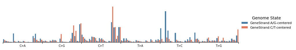
Strand-conditioned signatures
Pass a strand feature name to reveal transcriptional or replicational strand asymmetry.
[5]:
mu.pl.plot_component(data, components[0], 'GeneStrand')
[5]:
<Axes: >
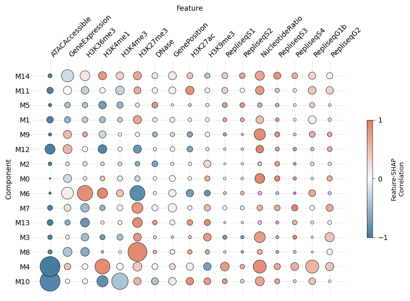
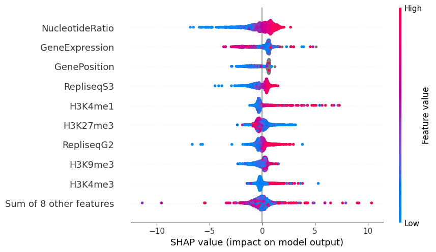
3. SHAP Feature Importance
SHAP values reveal which genomic features push each locus toward or away from a component. plot_shap_summary produces a beeswarm-style dot-plot: rows are features, color encodes feature value, and horizontal position encodes impact on the log mutation rate.
[6]:
mu.pl.plot_shap_summary(data, scale=40, max_size=20, figsize=(10, 6))
[6]:
<Axes: xlabel='Feature', ylabel='Component'>
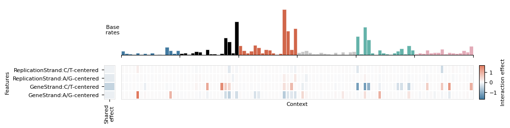
[8]:
# Feature interaction matrix for a single component
mu.pl.plot_interaction_matrix(data, components[0])
None
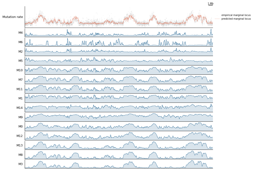
4. Genome-Browser Track Views
The track-plot module builds composable genome-browser figures. Here we compare predicted vs observed mutation rates and per-component rates over a 5 Mb window on chr2.
[12]:
view = tr.make_view(data, 'chr2:10000000-55000000')

def config(view, scalebar_bp):
    return (
        tr.scale_bar(scalebar_bp, scale='mb'),
        tr.tracks.plot_marginal_observed_vs_expected(view, pred_smooth=3, smooth=3, height=1.25),
        tr.plot_component_rates(view, *tr.order_components(data)),
        tr.spacer(0.2),
    )

tr.plot_view(config, view, scalebar_bp=1_000_000, width=10)
None
INFO Mutopia Found 6767/388247 regions matching query.
5. Exporting SHAP Explanations
SHAP Explanation objects can be retrieved for downstream analysis.
[13]:
import shap

explanation = mu.gt.get_explanation(data, component=components[0])
shap.plots.beeswarm(explanation)
Next steps
Tutorial 5: Annotating VCFs — apply the trained model to assign each mutation in a VCF to a component and estimate per-sample signature fractions.
Explore
mu.gt.rename_componentsto give components biologically meaningful names.Try
mu.gt.slice_regionsto focus analysis on a specific gene or locus.